|
METHODOLOGICAL NOTE ON THE STANDARD SAMPLE
THE UTILIZATION OF THE STANDARD SAMPLE: AN OVERVIEW
KEY VARIABLES AND THEIR FREQUENCY DISTRIBUTION
PROCEDURES AND STATISTICS IN THE CAUSAL DIAGRAMS
SELECTED REFERENCES AND COMMENTS
Each time I presented the findings from the Standard Sample I discussed in the text and in the "Selected References and Comments" section of the relevant chapter the specific variables used and some of the problems involved. Thus, I have discussed some of the validity and reliability problems of the Standard Sample data. Nevertheless, it is necessary to do three more things: (1) present an overview of the Standard Sample data and how I utilized them; (2) list the codebook wording of the variables used and their frequency breakdown, and (3) give the reader a matrix of the correlations of these variables, and more specific statistical data on the five causal diagrams in the book. This will afford you a better understanding of my findings and, in addition, it will make it much easier for those who desire to replicate or expand upon my findings.
THE UTILIZATION OF THE STANDARD SAMPLE:
AN OVERVIEW
By now the reader is aware that the Standard Sample is a subset of the Ethnographic Atlas. In 1969 Murdock and White selected what they felt were the best-described 186 nonindustrialized cultures representative of the six major culture regions of the world.1 The sample cultures divide as follows into these six regions:
Sub-Saharan Africa: 28 Societies
Circum-Mediterranean: 28 Societies
East Eurasia: 34 Societies
Insular Pacific: 31 Societies
North America: 33 Societies
South and Central America: 32 Societies
These societies were selected by the quality of the ethnographic coverage. The attempt was also made to avoid societies with a great deal of historical contact with each other in order to gain a more representative and broader view of the culture area. The societies chosen represented 51 independent linguistic families. The major types of subsistence in the Standard Sample is representative of those in the nonindustrialized world in general.
To avoid acculturation effects from contact with Europeans, the societies are described at the earliest period for which satisfactory ethnographic data are available. Most of the societies were studied between 1851 and 1950. For an exact location of the societies I suggest looking at the maps in the original article by Murdock and White.
The reader should bear in mind that these 186 societies represent the nonindustrialized societies of the world. No comparable sample of industrialized societies with similar information is available. In this book I have utilized small samples of industrialized societies or individual society studies in order to develop my ideas on the industrialized world. In addition, I have used some well-described nonindustrialized societies not included in this Standard Sample. Some, like the Sambia, were only very recently studied and were therefore not in the Standard Sample. Of course, those additional nonindustrialized societies were not part of the five causal diagrams I presented. They were brought into my discussions because they were good-quality ethnography and they had special value for our understanding human sexuality cross-culturally. I began to use the Standard Sample to examine some general causal notions that I had developed from my own in-depth reading of industrialized and nonindustrialized societies. I do not want to exaggerate the importance of the Standard Sample data for my theory. Although it surely added a great deal to my knowledge, my goal was the sociological understanding of human sexuality, and that extends far beyond the confines of the data in the Standard Sample.
My approach to the data in the Standard Sample was to select those coded variables that were most relevant for searching out the societal linkages of sexuality. In many cases I started by examining a variety of variables and selected from those the ones that seemed most appropriate. In some instances, as mentioned in previous chapters, I found codes that contradicted each other. In such cases I sought to find the codes that seemed the most valid. I arrived at this judgment, when possible, by checking "known cases." If I knew some cultures very well, for example, I would see how each source had coded those cultures and choose the source that conformed most closely to my conception of those societies. In other instances I chose on the basis of which source provided the most complete set of coded categories. In yet others I would choose on the basis of which source coded a sufficient number of societies for me to carry out the necessary statistical analysis.
On occasion I had to exclude variables that were measured inappropriately for testing my hypotheses. I had, for example, to drop a measure of male dominance because that measure included rape frequency in the society as an index of male dominance. This made it impossible for me to examine whether male dominance was related to rape frequency. In some cases I dropped measures because they did not distinguish males from females on behavior or attitude measures of sexuality. Knowing that most societies have noticeable elements of a double standard in sexuality, I could not confidently use a measure of sexuality that did not yield separate information on males and females.
In all these ways I was using my own knowledge and my own judgment in the selection of variables. However, the reader should not be too alarmed at my possible bias because the number of variables on sexuality was so small that in most instances I had to take what was available and no choice was possible. I will present here the variables I found most useful in my analysis. Those who wish can go to the original sources to seek for additional variables and make their own validation judgments.
KEY VARIABLES AND THEIR FREQUENCY DISTRIBUTION
I list here the name of the variable as given in the original codebook of the author or authors and follow it in parentheses by the name I used for it in this book. All variables have been arranged so that the categories are coded from low on the variable to high on the variable when applying my label for the variable. The variable wording is from the original sources, as are the answer categories, except in those cases where the categories consisted of a large number of numerical scores (interval data). In those instances, for simplicity sake, I have trichotomized the answer categories. I list the frequency distribution of responses for each category of each variable. Finally, I place an identification letter in front of each variable number so the reader can easily note the source of that variable.2 For the Standard Sample, in front of the variable number I place the letters SS; for Broude, B; for Whyte, W; for Ross, R; for Hupka, H; and for Sanday, S.
PERCENTAGE
NUMBER OF OF ALL
SOCIETIES SOCIETIES
CODED CODED
____________________________________________________________________________
(SS)l. NON-MATERNAL RELATIONSHIPS-INFANCY (MOTHER-INFANT INVOLVEMENT)
a. Most care, except nursing, is by others 1 0.6
b. Mother's role is significant but less than all other combined2 1.2
c. Mother provides half or less of the care 10 6.2
d. Principally mother, other have important roles 63 38.9
e. Principally mother, others have minor roles 81 50.0
f. Almost exclusively the mother 5 3.1
Total Number of Societies Coded 162 100.0
(SS)2. ROLE OF FATHER: INFANCY (FATHER-INFANT INVOLVEMENT)
a. No close proximity 8 5.2
b. Rare instances of close proximity 27 17.5
c. Occasional or irregular close proximity 72 46.8
d. Frequent close proximity 44 28.6
e. Regular, close relationship or companionship 3 1.9
Total Number of Societies Coded 154 100.0
(SS)3. MARITAL RESIDENCE AND DESCENT MALE KIN GROUPS)
(The above variable was coded by combining the responses to the marital residence and descent variables so that a society that was neither patrilocal or patrilineal received a low code; a society that was either patrilocal or patrilineal but not both received a medium code; and a society that was both patrilocal and patrilineal received a high code.)
a. Low on male kin groups 62 33.3
b. Medium on male kin groups 53 28.5
c. High on male kin groups 71 38.2
Total Number of Societies Coded 186 100.0
(SS)4. WILDPLANTS, HUNTING, FISHING, ANIMAL HUSBANDRY, AGRICULTURE (EXTENT OF AGRICULTURE)
(This variable was coded from the specific codes for the above-listed five types of subsistence in order to derive those societies in which agriculture was dominant over all other types of subsistence.)
a. Agriculture not greater than other forms of subsistence 59 33.3
b. Agriculture greater than other forms of subsistence 118 66.7
Total Number of Societies Coded 177 100.0
(SS)5. CLASS STRATIFICATION (CLASS STRATIFICATION)
a. Absence among freemen 76 41.3
b. Wealth distinctions 42 22.8
c. Elite (based on control of land or other resources) 3 1.6
d. Dual (hereditary aristocracy) 38 20.7
e. Complex (social classes) 25 13.6
Total Number of Societies Coded 184 100.0
(SS)6. NORMS OF PREMARITAL SEX BEHAVIOR OF GIRLS (FEMALE PREMARITAL HETEROSEXUAL PERMISSIVENESS)
a. Insistence on virginity 38 30.9
b. Prohibited but weakly censured and not infrequent 32 26.0
c. Allowed, censured only if pregnancy results 17 13.8
d. Trial marriage, promiscuous relations prohibited 3 2.4
e. Freely permitted, even if pregnancy results 33 26.8
Total Number of Societies Coded 123 100.0
The preceding six variables came from the Standard Sample.3 As the reader can see, there was only one direct question on sexuality. Clearly, I needed more sources, and so I went to the ethnographic literature to search for those who might have added new codes for the cultures in the Standard Sample. I came across five such sources. I next list the key variables from those sources, starting with Broude.4
(B)7. FREQUENCY OF PREMARITAL SEX (MALE) (MALE PREMARITAL HETEROSEXUAL FREQUENCY)
a. Uncommon: males rarely or never engage in premarital sex 13 12.7
b. Occasional: some males engage in premarital sex but this is not
common or typical 11 10.8
c. Moderate: not uncommon for males to engage in premarital sex 18 17.6
d. Universal or almost universal: almost all males engage in
premarital sex 60 58.8
Total Number of Societies Coded 102 100.0
(B)8. FREQUENCY OF EXTRAMARITAL SEX (MALE) (MALE EXTRAMARITAL HETEROSEXUAL FREQUENCY)
a. Uncommon: men rarely or never engage in extramarital sex 10 19.6
b. Occasional: men sometimes engage in extramarital sex, but
this is not common 6 11.8
c. Moderate: not uncommon for men to engage in extramarital sex 29 56.9
d. Universal or almost universal: almost all men engage in
extramarital sex 6 11.8
Total Number of Societies Coded 51 100.0
9. FREQUENCY OF EXTRAMARITAL SEX (FEMALE) (FEMALE EXTRAMARITAL HETEROSEXUAL FREQUENCY)
a. Uncommon: women rarely or never engage in extramarital sex 15 28.3
b. Occasional: women sometimes engage in extramarital sex, but
this is not common 9 17.0
c. Moderate: not uncommon for women to engage in
extramarital sex 23 43.4
d. Universal or almost universal: almost all women engage in
extramarital sex 6 11.3
Total Number of Societies Coded 53 100.0
(B)10. FREQUENCY OF RAPE (HETEROSEXUAL RAPE FREQUENCY)
a. Absent 8 25.8
b. Rare: isolated cases 10 32.3
c. Common: not atypical 13 41.9
Total Number of Societies Coded 31 100.0
(B)11. FREQUENCY OF HOMOSEXUALITY (FREQUENCY OF HOMOSEXUAL BEHAVIOR)
a. Absent, rare 40 58.0
b. Present, not uncommon 29 42.0
Total Number of Societies Coded 69 100.0
The next two variables come from Whyte.
(W)12. IS THERE A GENERALLY HIGH VALUE PLACED ON MALES BEING AGGRESSIVE, STRONG, AND SEXUALLY POTENT (MACHISMO)? (MACHISMO EMPHASIS)
a. Little or no emphasis 22 27.2
b. Moderate emphasis 33 40.7
c. Marked emphasis 26 32.1
Total Number of Societies Coded 81 100.0
(W)13. IS THERE A CLEARLY STATED BELIEF THAT WOMEN ARE GENERALLY INFERIOR TO MEN? (BELIEF IN FEMALE INFERIORITY)
a. No such belief 66 71.0
b. Yes 27 29.0
Total Number of Societies Coded 93 100.0
The next code comes from Ross.
(R)14. LOCAL CONFLICT; PHYSICAL FORCE; INTERNAL WARFARE; EXTERNAL WARFARE (VIOLENCE)
(This is a combined variable composed of the four variables listed. It was composed by giving one point for each of the four questions answered with a high response. See the specific reference from Ross in note 3 for the exact wording of each of the four questions. I counted a high response for Local Conflict as categories 1 and 2; a high response for Physical force as category a high response for Internal Warfare as Categories 1 and 2; and a high response for External Warfare as category 1.)
a. Lowest 21 23.3
b. Low 24 26.7
c. Low moderate 20 22.2
d. High moderate 16 17.8
e. High 9 10.0
Total Number of Societies Coded 90 100.0
The next six variables are from Hupka.
(H)15. WIFE'S SEXUAL JEALOUSY (WIFE'S SEXUAL JEALOUSY)
(Codes go from low to high on a scale of zero to 36 according to the severity of punishment for the person involved weighted by the impact on the marriage. For convenience sake, I trichotomize the scores here. In the regression runs all such interval variables were, of course, run fully open.5
a. Low = 0-12 9 23.1
b. Medium = 13-24 24 61.5
c. High = 25-36 6 15.4
Total Number of Societies Coded 39 100.0
(H)16. HUSBAND'S SEXUAL JEALOUSY (HUSBAND'S SEXUAL JEALOUSY)
(Coded the same as question 15.)
a. Low = 0-12 8 10.0
b. Medium = 13-24 27 33.8
c. High = 25-36 45 56.2
Total Number of Societies Coded 80 100.0
(H)17. PROPERTY (IMPORTANCE OF PROPERTY)
(This is coded from zero to 36 depending on the importance placed on property. For convenience sake, I trichotomize the scores here.)
a. Low = 0-12 19 23.7
b. Medium = 13-24 40 50.0
c. High = 25-36 21 26.3
Total Number of Societies Coded 80 100.0
(H)18. PROGENY (EMPHASIS ON PROGENY)
(This variable measures the emphasis on legitimate children and their importance to parents. It is measured by scores of 0-36. For convenience sake, I trichotomize the results here.)
a. Low = 0-12 20 25.0
b. Medium = 13-24 37 46.3
c. High = 25-36 23 28.7
Total Number of Societies Coded 80 100.0
(H)19. PAIRBONDING (IMPORTANCE OF MARRIAGE)
(This variable measures the emphasis placed on marriage in a society. It uses a scale of 0-36. For simplicity sake, I trichotomize the responses here.)
a. Low = 0-12 19 23.7
b. Medium = 13-24 36 45.0
c. High = 25-36 25 31.3
Total Number of Societies Coded 80 100.0
(H)20. SEXUAL GRATIFICATION (HETEROSEXUAL RESTRICTIVENESS)
(This variable measures restrictions on premarital, extramarital, and postmarital heterosexuality on a scale of 0-36. For simplicity sake, I trichotomize the responses here.)
a. Low = 0-12 25 31.3
b. Medium = 13-24 23 28.8
c. High = 25-36 32 40.0
Total Number of Societies Coded 80 100.00
The final set of questions comes from Sanday.
(S)21. AGRICULTURE (PREVALENCE OF AGRICULTURE)
(This variable was adopted by Sanday from the Standard Sample data.)
a. Not practiced 31 19.9
b. Practiced but confined to nonfood crop 3 1.9
c. Unimportant, less than 10% 17 10.9
d. Significant, more than 10% but less than any other 8 5.1
e. More than any other but less than 50% 34 21.8
f. More than all other subsistence techniques combined 63 40.4
Total Number of Societies Coded 156 100.0
(S)22. SEGREGATED FEMALE TECHNOLOGICAL ACTIVITIES (SEGREGATED FEMALE TECHNOLOGY)
(This variable uses a 50-item scale devised by G.P. Murdock and C. Provost and measures the percentage of all technological activities performed predominantly or exclusively by females.6 Sanday's scores run from 9 to 73. For the sake of convenience, I have trichotomized the item here.)
a. Low = 9-30 36 21.1
b. Medium = 31-52 101 64.7
c. High = 53-73 19 12.2
Total Number of Societies Coded 156 100.0
(S)23. SEXUALLY INTEGRATED TECHNOLOGICAL ACTIVITY (GENDERINTEGRATED TECHNOLOGY)
(This variable measures the percentage of all technological activities equally performed by both genders. It uses the same scale as in variable 22. Sanday's scores range from zero to 35. For convenience, I have trichotomized the responses here.)
a. Low = 0-12 113 72.4
b. Medium = 13-24 38 24.4
c. High = 25-35 5 3.2
Total Number of Societies Coded 156 100.0
(S)24. STRUCTURE(S) WHERE MALES CONGREGATE ALONE, OR MALES OCCUPY SEPARATE PART OF HOUSEHOLD, OR SHARP CEREMONIAL SEGREGATION OF THE SEXES (MALE STRUCTURES)
a. Absent 24 21.6
b. Present 87 78.4
Total Number of Societies Coded 111 100.0
(S)25. IDEOLOGY OF MALE TOUGHNESS, MACHISMO (MACHO)
a. Absent 21 19.4
b. Present 87 80.6
Total Number of Societies Coded 108 100.0
(S)26. INCIDENCE OF RAPE-OR EVIDENCE OF RAPE AS BEING AN ACCEPTED PRACTICE (HETEROSEXUAL RAPE PRONENESS)
a. Never, rare 45 47.4
b. Reported as present, no report of frequency or suggestion that
incidence is moderate; description such that clearly
cannot be classified as rare 33 34.7
c. Institutionalized (rape an accepted practice which is used
to punish women or is part of a ceremony) 17 17.9
Total Number of Societies Coded 95 100.0
(S)27. DEGREE OF INTERPERSONAL VIOLENCE (INTERPERSONAL VIOLENCE)
a. Mild or absent 44 33.6
b. Moderate 46 35.1
c. Strong 41 31.3
Total Number of Societies Coded 131 100.0
(S)28. FEMALE STATUS SCALE SCORE (FEMALE STATUS)
(This is basically a measure of the degree to which females produce subsistence and possess some power outside the domestic sphere. I have provided arbitrary labels.)
a. Lowest 11 8.3
b. Low 9 6.8
c. Low Moderate 5 3.8
d. Moderate 13 9.8
e. High Moderate 23 17.3
f. High 41 30.8
g. Highest 31 23.3
Total Number of Societies Coded 133 100.0
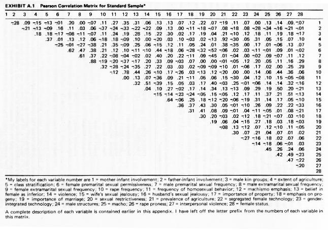
These 28 variables are the major ones referred to in this book. Sixteen of them comprise the variables in the causal diagrams.7 Twelve other variables are here because they are mentioned in the book in some significant fashion. I have two measures of the presence of agriculture, for example, for that is an important causal variable. I checked out my statements on the role of agriculture using both of them and thereby increased the confidence in the results. The same is true of the two measures of rape, violence, machismo, female status, and male kin groups. The precise variable I ended up using can be discerned by the variable label in the diagram.
There are also variables that were not so useful but are important in my discussion of findings. The sexual restrictiveness variable of Hupka, for example, tried to cover too many areas of sexuality with one measure. Since I discuss the problems with this variable in Chapter 3, I felt it belonged here for the reader to see its composition. The progeny variable of Hupka did not work out as an explanatory factor either, but it is included because many people believe that jealousy is based upon a fear of illegitimate offspring. The lack of support for that view in the progeny measure is important to recognize, and so I included it here for emphasis and possible further testing by others. In addition, I did not find Sanday's female status measure very useful and used Whyte's measure instead, but I still include both here. I include two measures of violence, for the results differ - as I mention in Chapter 7depending on which one you use.
In sum, then, the presence of a variable in this appendix does not mean it is being recommended. Rather, it is present if it is seen as important in the checking of the explanations tested in this book. These 28 were selected from a much larger number of variables after a long series of careful checks. It is hoped that some of the readers will continue to mine these data together with the new data that come forth regularly in this field.
PROCEDURES AND STATISTICS
IN THE CAUSAL DIAGRAMS
I started my analysis of the data by examining bivariate tables of these 28 variables and many others. My initial objective was to search for patterned ways each variable related to the others and thereby derive additional plausible hypotheses to test. To illustrate, it was from such examination that I noted the ways in which the various measures of male power seemed strongly associated with the measures of sexuality and consequently formulated some power explanations that became part of the causal diagrams later tested.
I examined many of these associations using other variables as controls to see if the relationship was general or limited to specific social contexts. I noted, for example, that an emphasis on male kin groups was associated with a belief in female inferiority, and I checked to see if this held up in polygamous as well as in monogamous societies, in unstratified as well as stratified societies, and so on. This relationship held up in all these societal contexts. This finding itself required the development of reasons for the broad scope under which the relationship of the presence of male kin groups associated with a belief in female inferiority.
The next step was to test some relationships involving more than two variables. Here, I soon ran into the problems associated with missing data. The reader can note the large differences in the number of societies coded on each of the 28 variables-the range being from 31 to 186 societies. This means that if you ran a traditional multiple regression you would only retain the lowest number of societies coded on any of the variables used in the regression. The missing-data problem also meant that you could not utilize as many variables in a single multiple regression as your theoretical interests might dictate; the more variables used, the more likely you will reduce the number of societies that have all of them coded.
I utilized some ways of minimizing these limitations. First, I did all my multiple regressions using both listwise and pairwise deletion. Listwise deletion, the traditional approach, reduces the total number of cases to that of the least answered variable; but pairwise deletion takes each two-variable regression independently and, therefore, does not drop those cases that have not been coded on all the variables. I always compared the results of both deletion methods, although for the diagrams in the book I used the pairwise deletion results. In the majority of cases, no difference was evident in the listwise and pairwise results.8 That is important because it increased my confidence in my results.
In addition, I also broke down my causal analysis into smaller segments than I otherwise would. There are 16 different variables in my five causal diagrams. Had the number of cases with information permitted, I would have tried to develop one causal diagram involving most of them; but there was no way that I could really test such a large diagram using the number of responses I had on each variable. Instead, my diagrams include a total of between 4 and 7 variables. However, the causal diagrams I used did have some variables in common, and thus one can easily speculate as to how two or more such causal patterns might fit together.
To begin with I did only regular multiple regressions of the variables in each of the five sets that were to become the five diagrams in the book. This enabled me to note what the net effect of each variable was on the dependent variable in that set. Then I thought that it would be much more meaningful if, in addition, I could test some ideas concerning the temporal sequence of influence among the several variables in each set of variables. So, I designed some causal sequences asserting a temporal order among the variables. The five causal diagrams in this book present the results of a series of multiple regressions aimed at discerning if the actual relationships among the variables fit into those proposed causal patterns. Such causal diagrams are helpful in building explanations much more than using only one multiple-regression analysis for each set of variables. There are other analysis techniques besides multiple regression which I might have tried but the missing data problem would interfere there also. Further, these data are crude measures and I felt that it would be best to not become too technically involved but rather to do a careful first examination of these data and leave it to others to proceed beyond that if they wish.
As a general background of the causal analysis it may be helpful to examine the bivariate correlations among the variables in any particular diagram. As an aid in doing this I present the correlation matrix for all 28 variables in Exhibit A. The reader may be interested in examining the correlations between variables supposedly measuring the same concept. The reader can also note how a particular bivariate correlation holds up when it is inserted into a multiple-regression analysis in the diagrams.
Following the matrix are five tables, one for each of the five diagrams. The relative strength of each relationship and its statistical probability is listed for each regression in each diagram. The first regression in each table is all one would have had if simple multiple regression were used in place of path analysis. It is important to present this information so as to further specify the nature of the support for these causal diagrams.9 Causal relationships are not something that one "proves"; rather, one examines proposed causal relationships to see how well they meet various statistical tests. If they are not shown to be in error by these tests, then our confidence is increased, but we never reach certainty.
Even the nontechnically trained reader can gain additional information from these tables. I suggest first looking down the column headed "significance level" in each of the five tables. If the notation there is listed as .10 or less, the relationship is considered a rare enough event to be called significant. Those relationships that met this statistical test appear on my chapter diagram represented by a line with an arrow connecting the two variables involved. You will note that many of the possible relationships do not come out significant. They were not all expected to come out significant. Rather, I designed causal diagrams, close to the final ones presented in the book, and expected only certain "paths" or relationships to come out significant.
 |
The "path coefficients" column in Tables A.1 to A.5 presents the standardized regressions (called betas) and allows one to judge the relative strength of relationships in any one diagram. The higher the beta, the stronger that particular relationship. Each table has between 3 to 6 dependent variables and each of them have one or more predictor variables in the next column. There is a beta for each predictor variable with each dependent variable. There is also an "R Sq" for each regression on a dependent variable. R Sq stands for the amount of variance in the dependent variable explained by all the predictor variables. That measure varies
TABLE A.1 Significance Levels and Path Coefficients for Diagram 3.1 on Husband's Sexual Jealousy*
TABLE A.2 Significance Levels and Path Coefficients for Diagram 3.2 on Wife's Sexual Jealousy*
 |
from zero to 1.0, and the higher it is, the more variance explained in the dependent variable. The more variance explained by the independent or predictor variables, the more accurately we could predict change in the dependent variable. My major interest here is theoretical and not prediction, and therefore I do not stress how much variance I explain but rather whether the relationships came out significant and fit with a particular explanatory schema.10 I realize some of this may be complex for those who haven't used these techniques. Any standard statistics text will be quite helpful.
Basically, a causal diagram is an attempt to portray accurately the actual correlations among the variables. I could have presented additional statistics and thereby further detailed the nature of my statistical findings. I refrained from doing this because I feel the data from the Standard Sample that I am using are crude, and it is best to treat the analysis of such data as a pilot study for arriving at causal notions that will be tested further in future research. Perhaps others will be able to test my explanations more precisely with additional data and codes.
I hope some of the readers will have sufficient interest to further explore my findings on the Standard Sample. New data codes are developed all the time. The lack of detailed analysis of sexual customs by many ethnographers has led to sexuality, even for the Standard Sample societies, being inadequately described. This inadequate coverage of sexuality inevitably leads to coding problems because with inadequate data, reliable and valid codes are indeed hard to come by. I tried to deal with this problem by selecting the best variables available, but there still are many problems. However, my reading of current anthropological work indicates that this situation is being remedied. In part this is so because of the greater influence today by anthropologists with an interest in gender and sexuality. For industrialized societies we also have need for a firmer database upon which to examine our explanations. Here, too, I am encouraged by some of the recent research that even the U.S. government agencies have undertaken.11
I wish to end this technical appendix by reminding the reader that the ultimate goal of scientific research is explanation. So, if the details of the data overwhelm you once in a while, remember that they are the bases for developing more accurate and useful explanations of human sexuality.
TABLE A.3 Significance Levels and Path Coefficients for Diagram 4.1 on Female
Gender Inequality*
TABLE A.4 Significance Levels and Path Coefficients for Diagram 6.1 on Male
Homosexual Behavior*
TABLE A.5 Significance Levels and Path Coefficients for Diagram 7.1
on Rape Proneness*
SELECTED REFERENCES AND COMMENTS
1. Murdock, George P., and Douglas R. White, "Standard Cross Cultural Sample," Ethnology, vol. 8 (October 1969), pp. 329-369.
2. The sources for the 28 variables are
Whyte, Martin King, "Cross-cultural Codes Dealing with the Relative Status of Women," Ethnology, vol. 17 (April 1978), pp. 211-237.
Broude, Gwen J., and Sarah J. Greene, "Cross-cultural Codes on Twenty Sexual Attitudes and Practices," Ethnology, vol. 15 (October 1976), pp. 409-429.
Ross, Marc Howard, "Political Decision Making and Conflict: Additional Cross-cultural Codes and Scales," Ethnology, vol. 22 (April 1983), pp. 169-192.
The raw data and codes from Hupka and Sanday were sent to me upon request. They are unpublished, but these authors have analyzed these data in the following publications:
Sanday, Peggy Reeves, "The Socio-cultural Context of Rape: A Cross-cultural Study," Journal of Social Issues, vol. 37, no. 4 (October 1981), pp. 5-27.
Hupka, Ralph, "Cultural Determinants of Jealousy," Alternative Lifestyles, vol. 4 (August 1981), pp. 310-356.
The data from the Standard Sample were purchased on a computer tape from HRAF (the Human Relations Area Files) in New Haven, Connecticut. Anyone wishing these data can contact HRAF, and anyone wishing the Sanday or Hupka data will have to contact them for permission. Sanday is a professor at the University of Pennsylvania, and Hupka is a professor at California State University in Long Beach.
3. Variables SS4, SS5, and SS6 are codes from the Ethnographic Atlas. Since the Standard Sample is a subset of the atlas, any codes available for the atlas can be used on the Standard Sample.
4. The frequencies given for each variable are in a few instances slightly different than those presented by the sources I consulted. I carefully checked such differences and reconciled them as best I could. They were differences only of one or two cases in a particular category of response.
I should clarify further the reasons for many of the codes not being available for all 186 societies. Whyte took a 50% sample of the 186 societies and thus chose to use only 93 of the societies. Ross also chose a 50% sample of the 186 societies in his coding and found 3 of them uncodable and so ended up with 90 societies. Hupka obtained his societies from the HRAF files and came up with only 80 cultures that were in the Standard Sample. Sanday found only 156 societies of the Standard Sample were sufficiently codable for her purposes. Broude also found that many of the societies in the Standard Sample lacked sufficient information on enough of her variables to be useful. She used between 31 and 102 societies for the codes I used in this book.
5. Hupka's coding schema is described in the following paper:
Hupka, Ralph B., and James M. Ryan, "The Cultural Contribution to Emotions: Cross-cultural Aggression in Romantic Jealousy Situations." Paper presented at the meetings of the Western Psychological Association, Los Angeles, 1981.
6. Murdock, George P., and Caterina Provost, "Factors in the Division of Labor by Sex: A Cross-cultural Analysis," Chapter 10 in Hebert Barry and Alice Schlegel, (ed.), Cross-cultural Samples and Codes. Pittsburgh: University of Pittsburgh Press, 1980.
7. The numbers of the variables that were not used in any of the diagrams are 7, 8, 9, 10, 18, 20, 21, 22, 23, 24, 27, and 28.
8. There were 53 path coefficients checked in these five diagrams. Listwise and pairwise deletion methods agreed on 46 of them. There are problems with using listwise or pairwise deletion procedures with these data. But my use of both and final reliance on pairwise is in line with current views. See:
Anderson, Andy B., A Basilevsky, and D.P.J. Hum, "Missing Data: A Review of the Literature," Chapter 12 in Peter H. Rossi, James D. Wright, and Andy B. Anderson (eds.), Handbook of Survey Research. New York: Academic, 1983.
9. In some instances the dependent variables I used in my regression analysis were dichotomies. I did use other statistical techniques, including tabular analysis, to check for any distortion this may have produced. As far as I could tell, the use of dichotomies as dependent variables did not distort my findings.
10. All my causal diagrams assume asymmetrical relationships, that is, oneway causation. Of course, reality may well in some cases involve two-way causation or a "feedback loop." The assumption of asymmetry is simply a convenient way to make a first approximation in a causal diagram. I do not view it as the final word.
For the reader interested in the many intricate issues connected with causal analysis in the social sciences, I suggest the following brief selections:
Freese, Lee, (ed.) Theoretical Methods in Sociology. Pittsburgh: University of Pittsburgh Press, 1980.
Bailey, K.D., "Evaluating Axiomatic Theories," pp. 48-71 in E.F. Borgatta and G.W. Bohrnstedt (eds.), Sociological Methodology. San Francisco: Jossey-Bass, 1970.
Costner, H.L., and R. Leik, "Deductions from Axiomatic Theory," pp. 49-72 in H. Blalock, Jr. (ed.), Causal Models in the Social Sciences. Chicago: Aldine, 1971.
11. A recent government study, the National Survey of Family Growth (cycle 3), included within it questions on the timing of first sexual intercourse. Not too long ago the government would have avoided such questions. I consider this a very positive step toward improved knowledge regarding human sexuality. I believe it will aid us in dealing with the many problems related to sexuality. See
U.S. Department of Health and Human Services, National Center for Health Statistics, C.A. Bachrach and M.C. Horn, "Marriage and First Intercourse, Martial Dissolution, and Remarriage: U.S., 1982," no. 107. Hyattsville, Md.: Public Health Service, April 1985.
|